Page 178 - Principles of Applied Reservoir Simulation 2E

Part II: Reservoir Simulation 163

that are nearest neighbors to the central block along orthogonal Cartesian axes.
In Table 16-1, the central block is denoted by "C" and the nearest neighbor block
contributing to the standard finite difference calculation in 2D are denoted by
an asterisk. The five blocks comprise the five-point differencing scheme of the
2D Cartesian grid.
Table 16-1
Finite Difference Stencils
Block 1-1 I 1 + 1

J-l 9 # 9
J * C *

J + l 9 * 9

Reservoir simulators are usually formulated with the assumption that
diagonal blocks do not contribute because the grid is aligned along the principal
axes of the permeability tensor. Diagonal blocks are denoted by "9" in Table
16-1. The nine-point stencil includes all nine blocks in the calculation of flow
into and out of the central block. Grid orientation effects can be minimized, at
least in principle, if the diagonal blocks are included in the nine-point finite
difference formulation [for example, see Young, 1984; Hegre, etal, 1986: Lee,
et al., 1997]. This option is available in some commercial simulators. In 3D
models, the number of blocks needed to represent all adjacent blocks, including
diagonal terms, is 27. By contrast, only seven blocks are used in the conventional
formulation of a 3D finite difference model.
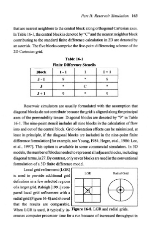
Local grid refinement (LGR)
LGR Radial Grid
is used to provide additional grid
definition in a few selected regions
of a larger grid. Raleigh [1991] com-
pared local grid refinement with a
radial grid (Figure 16-8) and showed
that the results are comparable.
When LGR is used, it typically in- Figure 16-8. LGR and radial grids,
creases computer processor time for a run because of increased throughput in