Page 105 - Probability and Statistical Inference

82 2. Expectations of Functions of Random Variables

Next, using the chain rule of differentiation, from (2.3.11) one obtains

Since M (0) = 1, from (2.3.11) it is obvious that dM (t)/dt, when evaluated
X
X
at t = 0, reduces to η = λ which matches with the expression of µ found earlier
1
in (2.2.18). Here is another way to check that the mean of the distribution is λ.
Also, the Theorem 2.3.1 would equate the expression of η or E(X ) with
2
2
2
2
d M (t)/dt , evaluated at t = 0. From (2.3.12) it should become obvious that
X
2
2
d M (t)/dt , evaluated at t = 0, should be η = λ + λ since M (0) = 1. Hence,
2
X
X
2
we have V(X) = E(X ) – µ = λ + λ – λ = λ. This again matches with the
2
2
2
2
2
expression of σ given in (2.2.18).
2.3.3 The Normal Distribution
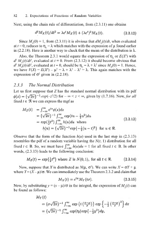
Let us first suppose that Z has the standard normal distribution with its pdf
2
exp(–z /2) for – ∞ < z < ∞, given by (1.7.16). Now, for all
fixed t ∈ ℜ we can express the mgf as
Observe that the form of the function h(u) used in the last step in (2.3.13)
resembles the pdf of a random variable having the N(t, 1) distribution for all
fixed t ∈ Β. So, we must have h(u)du = 1 for all fixed t ∈ Β. In other
words, (2.3.13) leads to the following conclusion:

Now, suppose that X is distributed as N(µ, σ ). We can write X = σY + µ
2
where Y = (X – µ)/σ. We can immediately use the Theorem 2.3.2 and claim that

Now, by substituting y = (x – µ)/σ in the integral, the expression of M (t) can
Y
be found as follows: