Page 108 - Probability and Statistical Inference

2. Expectations of Functions of Random Variables 85

so that d M (t)/dt , when evaluated at t = 0, reduces to α(1 + α)β . In view
2
2
2
X
of the Theorem 2.3.1, we can say that αβ is the mean of X and V(X) = E(X )
2
– µ = α(1 + α)β – µ = αβ . These same answers were derived earlier in
2
2
2
2
(2.2.39).
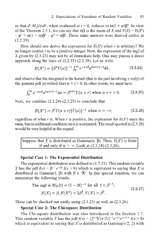
How should one derive the expression for E(X ) when r is arbitrary? We
r
no longer restrict r to be a positive integer. Now, the expression of the mgf of
X given by (2.3.23) may not be of immediate help. One may pursue a direct
approach along the lines of (2.2.35)-(2.2.38). Let us write
and observe that the integrand is the kernel (that is the part involving x only) of
the gamma pdf provided that α + r > 0. In other words, we must have

Next, we combine (2.3.24)-(2.3.25) to conclude that

regardless of what r is. When r is positive, the expression for E(X ) stays the
r
same, but no additional condition on α is warranted. The result quoted in (2.3.26)
would be very helpful in the sequel.

Suppose that X is distributed as Gamma(α, β). Then, E(X ) is finite
r
if and only if α > –r. Look at (2.3.24)-(2.3.26).

Special Case 1: The Exponential Distribution
The exponential distribution was defined in (1.7.23). This random variable
X has the pdf f(x) = β e –x/β I(x > 0) which is equivalent to saying that X is
–1
+
distributed as Gamma(1, β) with β ∈ ℜ . In this special situation, we can
summarize the following results.

These can be checked out easily using (2.3.23) as well as (2.3.26).
Special Case 2: The Chi-square Distribution
The Chi-square distribution was also introduced in the Section 1.7.
ν/2
This random variable X has the pdf f(x) = {2 Γ(ν/2)} e x I(x > 0)
–1 –x/2 (ν/2)–1
which is equivalent to saying that X is distributed as Gamma(ν/2, 2) with