Page 110 - Probability and Statistical Inference

2. Expectations of Functions of Random Variables 87

can claim that the random variable U and its distribution we have indicated are
unique. !
Example 2.4.2 Suppose that U is a random variable such that M (t) = 1/
U
16(1 + e ) . We can rewrite M (t) = (1/2 + 1/2 e ) which agrees with the ex-
t 4
t 4
U
pression of M (t) given by (2.3.5) where n = 4 and p = 1/2. Hence U must be
X
distributed as Binomial(4, 1/2) by the Theorem 2.4.1. !
Example 2.4.3 Suppose that U is a random variable such that M (t) =
U
exp{πt } which agrees with the expression of M (t) given by (2.3.16) with µ =
2
X
2
0, σ = 2π. Hence, U must be distributed as N(0, 2π). !
A finite mgf determines the distribution uniquely.
Before we move on, let us attend to one other point involving the moments.
A finite mgf uniquely determines a probability distribution, but on the other
hand, the moments by themselves alone may not be able to identify a unique
random variable associated with all those moments. Consider the following
example.
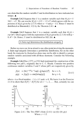
Example 2.4.4 Rao (1973, p.152) had mentioned the construction of the
following two pdf’s, originally due to C. C. Heyde. Consider two positive
continuous random variables X and Y whose pdf’s are respectively given by

where c is a fixed number, –1 ≤ c ≤ 1 and c ≠ 0. We leave it as the Exercise
2.4.4 to show that E[X ] = E[Y ] for all r = 1, 2, ... . But, certainly we can
r
r

Figure 2.4.1. The Two PDF’s from (2.4.1): (a) f(x) (b) g(y)
Where c = 1/2