Page 114 - Probability and Statistical Inference

2. Expectations of Functions of Random Variables 91

2.2.13 Suppose that X is a continuous random variable having its pdf f(x)
with the support χ = (a, b), –∞ ≤ a < b ≤ ∞. Additionally suppose that f(x) is
symmetric about the point x = c where a < c < b. Then, show that both the mean
and median of this distribution will coincide with c as long as the mean is finite.
{Hint: First show that the point of symmetry c for f(x) must be the midpoint
between a and b. Consider splitting the relevant integrals as the sum of the
integrals over the intervals (–∞, a), (a, c), (c, b) and (b, ∞). A word of caution
may be in order. A pdf may be symmetric about c, but that may not imply µ = c
simply because µ may not even be finite. Look at the Exercise 2.3.8.}
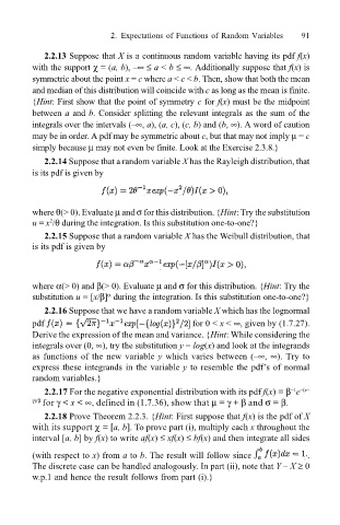
2.2.14 Suppose that a random variable X has the Rayleigh distribution, that
is its pdf is given by

where θ(> 0). Evaluate µ and σ for this distribution. {Hint: Try the substitution
2
u = x /θ during the integration. Is this substitution one-to-one?}
2.2.15 Suppose that a random variable X has the Weibull distribution, that
is its pdf is given by

where α(> 0) and β(> 0). Evaluate µ and σ for this distribution. {Hint: Try the
substitution u = [x/β] during the integration. Is this substitution one-to-one?}
α
2.2.16 Suppose that we have a random variable X which has the lognormal
pdf for 0 < x < ∞, given by (1.7.27).
Derive the expression of the mean and variance. {Hint: While considering the
integrals over (0, ∞), try the substitution y = log(x) and look at the integrands
as functions of the new variable y which varies between (–∞, ∞). Try to
express these integrands in the variable y to resemble the pdf’s of normal
random variables.}
2.2.17 For the negative exponential distribution with its pdf f(x) = β e
–1 –(x–
γ)/β for γ < x < ∞, defined in (1.7.36), show that µ = γ + β and σ = β.
2.2.18 Prove Theorem 2.2.3. {Hint: First suppose that f(x) is the pdf of X
with its support χ = [a, b]. To prove part (i), multiply each x throughout the
interval [a, b] by f(x) to write af(x) ≤ xf(x) ≤ bf(x) and then integrate all sides

(with respect to x) from a to b. The result will follow since .
The discrete case can be handled analogously. In part (ii), note that Y – X ≥ 0
w.p.1 and hence the result follows from part (i).}