
Page 119 - Probability and Statistical Inference
P. 119
96 2. Expectations of Functions of Random Variables
the process of evaluating the relevant integrals, try the substitution u = log(x).}
2.4.5 (Exercise 2.4.4 Continued) Suppose a random variable X has the
x exp[1/2(log(x)) ]I(x > 0). Show that the mgf
lognormal pdf f(x) = (2π) 1/2 1 2
of X does not exist. {Hint: In the process of evaluating the relevant integral,
one may try the substitution u = log(x).}
2.4.6 (Exercise 2.4.4 Continued) Consider the two pdfs f(x) and g(y)
with x > 0, y > 0, as defined in the Exercise 2.4.4 Let a(x) with x > 0 be any
other pdf which has all its (positive integral) moments finite. For example,
a(x) may be the pdf corresponding to the Gamma(α, β) distribution. On the
other hand, there is no need for a(x) to be positive for all x > 0. Consider now
two non-negative random variables U and V with the respective pdfs f (u)
0
and g (v) with u > 0, v > 0 where
0
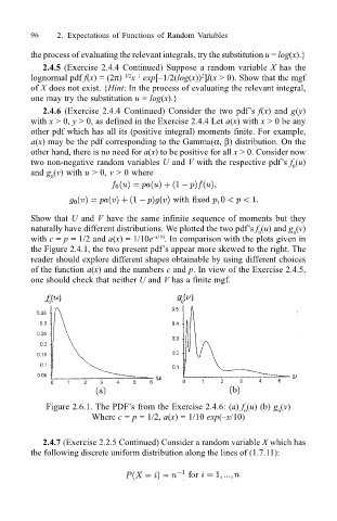
Show that U and V have the same infinite sequence of moments but they
naturally have different distributions. We plotted the two pdfs f (u) and g (v)
0
0
with c = p = 1/2 and a(x) = 1/10e x/10 . In comparison with the plots given in
the Figure 2.4.1, the two present pdfs appear more skewed to the right. The
reader should explore different shapes obtainable by using different choices
of the function a(x) and the numbers c and p. In view of the Exercise 2.4.5,
one should check that neither U and V has a finite mgf.
Figure 2.6.1. The PDFs from the Exercise 2.4.6: (a) f (u) (b) g (v)
0
0
Where c = p = 1/2, a(x) = 1/10 exp(x/10)
2.4.7 (Exercise 2.2.5 Continued) Consider a random variable X which has
the following discrete uniform distribution along the lines of (1.7.11):