Page 124 - Probability and Statistical Inference

3. Multivariate Random Variables 101

3.2.1 The Joint, Marginal and Conditional Distributions

Suppose that we have k(≥ 2) discrete random variables X , ..., X where X i
1
k
takes one of the possible values x belonging to its support χ , i = 1, ..., k.
i i
Here, χ can be at most countably infinite. The joint probability mass function
i
(pmf) of X = (X , ..., X ) is then given by
1 k
A function such as f(x) would be a genuine joint pmf if and only if the follow-
ing two conditions are met:

These are direct multivariable extensions of the requirements laid out earlier in
(1.5.3) in the case of a single real valued random variable.
The marginal distribution of X corresponds to the marginal probability
i
mass function defined by

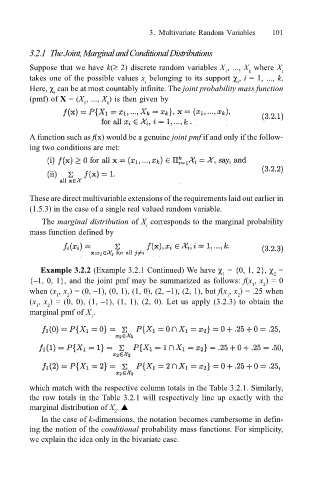
Example 3.2.2 (Example 3.2.1 Continued) We have χ = {0, 1, 2}, χ =
1 2
{–1, 0, 1}, and the joint pmf may be summarized as follows: f(x , x ) = 0
1
2
when (x , x ) = (0, –1), (0, 1), (1, 0), (2, –1), (2, 1), but f(x , x ) = .25 when
2
1
2
1
(x , x ) = (0, 0), (1, –1), (1, 1), (2, 0). Let us apply (3.2.3) to obtain the
1 2
marginal pmf of X .
1

which match with the respective column totals in the Table 3.2.1. Similarly,
the row totals in the Table 3.2.1 will respectively line up exactly with the
marginal distribution of X . !
2
In the case of k-dimensions, the notation becomes cumbersome in defin-
ing the notion of the conditional probability mass functions. For simplicity,
we explain the idea only in the bivariate case.