Page 126 - Probability and Statistical Inference

3. Multivariate Random Variables 103

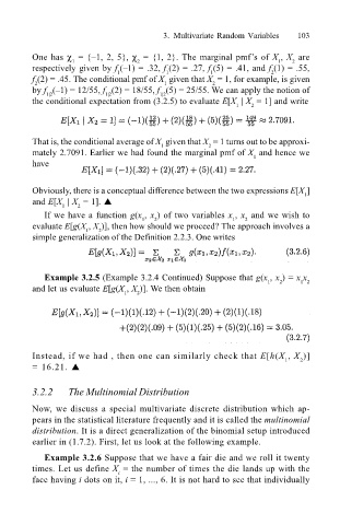
One has χ = {–1, 2, 5}, χ = {1, 2}. The marginal pmf’s of X , X are
2
1
1
2
respectively given by f (–1) = .32, f (2) = .27, f (5) = .41, and f (1) = .55,
2
1
1
1
f (2) = .45. The conditional pmf of X given that X = 1, for example, is given
2 1 2
by f (–1) = 12/55, f (2) = 18/55, f (5) = 25/55. We can apply the notion of
1|2
1|2
1|2
the conditional expectation from (3.2.5) to evaluate E[X | X = 1] and write
1 2
That is, the conditional average of X given that X = 1 turns out to be approxi-
2
1
mately 2.7091. Earlier we had found the marginal pmf of X and hence we
1
have
Obviously, there is a conceptual difference between the two expressions E[X ]
1
and E[X | X = 1]. !
1 2
If we have a function g(x , x ) of two variables x , x and we wish to
1
2
1
2
evaluate E[g(X , X )], then how should we proceed? The approach involves a
1
2
simple generalization of the Definition 2.2.3. One writes
Example 3.2.5 (Example 3.2.4 Continued) Suppose that g(x , x ) = x x
1 2
1
2
and let us evaluate E[g(X , X )]. We then obtain
1 2
Instead, if we had , then one can similarly check that E[h(X , X )]
1 2
= 16.21. !

3.2.2 The Multinomial Distribution
Now, we discuss a special multivariate discrete distribution which ap-
pears in the statistical literature frequently and it is called the multinomial
distribution. It is a direct generalization of the binomial setup introduced
earlier in (1.7.2). First, let us look at the following example.
Example 3.2.6 Suppose that we have a fair die and we roll it twenty
times. Let us define X = the number of times the die lands up with the
i
face having i dots on it, i = 1, ..., 6. It is not hard to see that individually