Page 123 - Probability and Statistical Inference

100 3. Multivariate Random Variables

independence are explained in the Section 3.7. The Section 3.8 summarizes
both the one- and multi-parameter exponential families of distributions. This
chapter draws to an end with some of the standard inequalities which are
widely used in statistics. The Sections 3.9.1-3.9.4 include more details than
Sections 3.9.5-3.9.7.

3.2 Discrete Distributions

Let us start with an example of bivariate discrete random variables.
Example 3.2.1 We toss a fair coin twice and define U = 1 or 0 if the i toss
th
i
results in a head (H) or tail (T), i = 1, 2. We denote X = U + U and X = U
1 1 2 2 1
– U . Utilizing the techniques from the previous chapters one can verify that
2
X takes the values 0, 1 and 2 with the respective probabilities 1/4, 1/2 and 1/
1
4, whereas X takes the values –1, 0 and 1 with the respective probabilities 1/
2
4, 1/2 and 1/4. When we think of the distribution of X alone, we do not worry
i
much regarding the distribution of X , i ≠ j = 1, 2. But how about studying the
j
random variables (X , X ) together? Naturally, the pair (X , X ) takes one of
1
2
1
2
the nine (= 3 ) possible pairs of values: (0, –1), (0, 0), (0, 1), (1, –1), (1, 0),
2
(1, 1), (2, –1), (2, 0), and (2, 1).
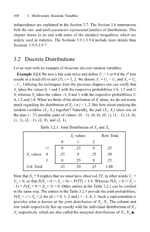
Table 3.2.1. Joint Distribution of X and X
1 2
X values Row Total
1
0 1 2
–1 0 .25 0 .25
X values 0 .25 0 .25 .50
2
1 0 .25 0 .25
Col. Total .25 .50 .25 1.00
Note that X = 0 implies that we must have observed TT, in other words U =
1
1
U = 0, so that P(X = 0 ∩ X = 0) = P(TT) = 1/4. Whereas P(X = 0 ∩ X =
2 1 2 1 2
–1) = P(X = 0 ∩ X = 1) = 0. Other entries in the Table 3.2.1 can be verified
1
2
in the same way. The entries in the Table 3.2.1 provide the joint probabilities,
P(X = i ∩ X = j) for all i = 0, 1, 2 and j = –1, 0, 1. Such a representation is
1
2
provides what is known as the joint distribution of X , X . The column and
1 2
row totals respectively line up exactly with the individual distributions of X ,
1
X respectively which are also called the marginal distributions of X , X .!
2 1 2