Page 154 - Probability and Statistical Inference
P. 154

3. Multivariate Random Variables  131

                                   Refer to (1.7.13), (1.7.20) and (1.7.31) as needed. Note that the
                           Theorem 3.5.3 really makes it simple to write down the marginal pdf’s in
                           the case of independence. !
                                  It is crucial to note that the supports χ ’s are assumed to
                                                                    i
                                 be unrelated to each other so that the representation given
                                by (3.5.6) may lead to the conclusion of independence among
                                   the random variables X ’s. Look at the Example 3.5.11
                                                        i
                                   to see what may happen when the supports are related.

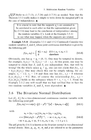
                              Example 3.5.11  (Examples 3.3.1 and 3.5.2 Continued) Consider two
                           random variables X  and X  whose joint continuous distribution is given by
                                            1     2
                           the following pdf:


                           Obviously, one has χ  = χ  = (0, 1). One may be tempted to denote,
                                               1
                                                   2
                           for example, h (x ) = 6, h (x ) = (1 – x ). At this point, one may be
                                         1  1      2  2         2
                           tempted to claim that X  and X  are independent. But, that will be
                                                  1      2
                           wrong! On the whole space χ  × χ , one can not claim that f(x , x )
                                                                                          2
                                                            2
                                                       1
                                                                                       1
                           =  h (x )h (x ). One may check this out by simply taking, for ex-
                              1  1  2  2
                           ample,  x  = 1/2,  x  = 1/4 and then one has  f(x ,  x ) = 0 whereas
                                   1         2                           1   2
                           h (x )h (x ) = 9/2. But, of course the relationship  f(x ,  x ) =
                                     2
                                                                                    1
                                                                                        2
                               1
                            1
                                  2
                           h (x )h (x ) holds in the subspace where 0 < x  < x  < 1. From the
                            1  1  2  2                                  1   2
                           Example 3.5.2 one will recall that we had verified that in fact the
                           two random variables X  and X  were dependent. !
                                                  1      2
                           3.6   The Bivariate Normal Distribution
                           Let (X , X ) be a two-dimensional continuous random variable with
                                 1
                                    2
                           the following joint pdf:
                            with

                           The pdf given by (3.6.1) is known as the bivariate normal or two-dimensional
                           normal density. Here, µ , µ , σ , σ  and ρ are referred to as the parameters
                                               1  2  1   2
   149   150   151   152   153   154   155   156   157   158   159