Page 159 - Probability and Statistical Inference

136 3. Multivariate Random Variables

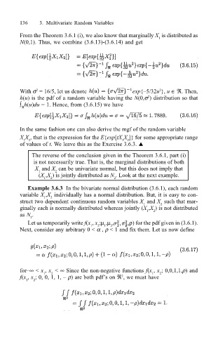
From the Theorem 3.6.1 (i), we also know that marginally X is distributed as
1
N(0,1). Thus, we combine (3.6.13)-(3.6.14) and get

With σ = 16/5, let us denote exp{–5/32u }, u ∈ ℜ. Then,
2
2
h(u) is the pdf of a random variable having the N(0,σ ) distribution so that
2
∫ h(u)du = 1. Hence, from (3.6.15) we have
ℜ

In the same fashion one can also derive the mgf of the random variable
X X , that is the expression for the E{exp[tX X ]} for some appropriate range
2
1
2
1
of values of t. We leave this as the Exercise 3.6.3. !
The reverse of the conclusion given in the Theorem 3.6.1, part (i)
is not necessarily true. That is, the marginal distributions of both
X and X can be univariate normal, but this does not imply that
1 2
(X ,X ) is jointly distributed as N . Look at the next example.
1 2 2
Example 3.6.3 In the bivariate normal distribution (3.6.1), each random
variable X ,X individually has a normal distribution. But, it is easy to con-
2
1
struct two dependent continuous random variables X and X such that mar-
2
1
ginally each is normally distributed whereas jointly (X ,X ) is not distributed
1
2
as N .
2
Let us temporarily write f(x , x ;µ ,µ , ρ) for the pdf given in (3.6.1).
2
2
1
1
Next, consider any arbitrary 0 < α , ρ < 1 and fix them. Let us now define
for–∞ < x , x < ∞ Since the non-negative functions f(x , x ; 0,0,1,1,ρ) and
1
2
2
1
2
f(x , x ; 0, 0, 1, 1, – ρ) are both pdf’s on ℜ , we must have
1 2