Page 163 - Probability and Statistical Inference

140 3. Multivariate Random Variables

which happens to be zero. Thus, we note that P {X > 4 | –2 ≤ X ≤ 2} ≠ P
1
2
{X > 4}. Hence, X and X are dependent variables. !
2 1 2
One can easily construct similar examples in a discrete
situation. Look at the Exercises 3.7.1-3.7.3.
Example 3.7.2 Suppose that Θ is distributed uniformly on the interval
[0, 2π). Let us denote X = cos(Θ), X = sin(Θ). Now, one has E[X ] =
1 2 1
Also, one can write E[X X ] =
1 2
. Thus,
Cov(X , X ) = E(X X ) – E(X )E(X ) = 0 – 0 = 0. That is, the correlation
2
1
2
1
1
2
coefficient ρ , is zero. But the fact that X and X are dependent can be
X1 X2
2
1
easily verified as follows. One observes that and hence condi-
tionally given X = x , the random variable X can take one of the possible
1
1
2
values, or with probability 1/2 each. Suppose that we
fix x = . Then, we argue that P{–1/4 < X < 1/4 | X = } = 0, but obvi-
1
1
2
ously P{–1/4 < X < 1/4} > 0. So, the random variables X and X are depen-
2
1
2
dent. !
Theorem 3.7.1 mentions that ρ , = 0 implies independence
X1 X2
between X and X when their joint distribution is N . But,
1
2
2
ρ , = 0 may sometimes imply independence between
X1 X2
X and X even when their joint distribution is different from
1 2
the bivariate normal. Look at the Example 3.7.3.
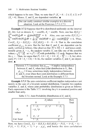
Example 3.7.3 The zero correlation coefficient implies independence not
merely in the case of a bivariate normal distribution. Consider two random
variables X and X whose joint probability distribution is given as follows:
1
2
Each expression in the Table 3.7.1 involving the p’s is assumed positive and
smaller than unity.
Table 3.7.1. Joint Probability Distribution of X and X
1 2
X values Row
1
0 1 Total
0 1 – p p + p 1 – p
1 1 2
X – p +p
2 1
values
1 p – p p p
2 2
Col. Total 1 – p p 1
1 1
Now, we have Cov(X , X ) = E(X X )–E(X )E(X ) = P{X = 1∩X = 1} –
2
1
1
1
2
1
2
2
P{X = 1} P{X = 1} = p – p p , and hence the zero correlation
1 2 1 2