Page 165 - Probability and Statistical Inference

142 3. Multivariate Random Variables

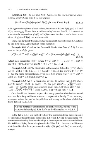
Definition 3.8.1 We say that f(x;θ) belongs to the one-parameter expo-
nential family if and only if we can express

with appropriate forms of real valued functions a(θ) ≥ 0, b(θ), g(x) ≥ 0 and
R(x), where χ ⊆ ℜ and Θ is a subinterval of the real line ℜ. It is crucial to
note that the expressions of a(θ) and b(θ) can not involve x, while the expres-
sions of g(x) and R(x) can not involve θ.
Many standard distributions, including several listed in Section 1.7, belong
to this rich class. Let us look at some examples.
Example 3.8.1 Consider the Bernoulli distribution from (1.7.1). Let us
rewrite the pmf f(x; p) as

which now resembles (3.8.1) where θ = p, a(θ) = 1 – θ, g(x) = 1, b(θ) =
–1
log{θ(1 – θ) }, R(x) = x, and Θ = (0, 1), χ = {0, 1}. !
Example 3.8.2 Let X be distributed as Poisson(λ), defined in (1.7.4) where
λ(> 0). With χ = {0, 1, 2, ...}, θ = λ, and Θ = (0, ∞), the pmf f(x; θ) = e θ /
–θ
x
–1
x! has the same representation given in (3.8.1) where g(x) = (x!) , a(θ) =
exp{–θ}, b(θ) = log(θ) and R(x) = x. !
Example 3.8.3 Let X be distributed as N(µ, 1), defined in (1.7.13) where
µ ∈ ℜ. With χ = ℜ, θ = µ, and Θ = ℜ, the pdf exp{–
2
1/2(x – θ) } has the same representation given in (3.8.1) where g(x) = exp{–
1/2x }, exp{–1/2θ }, b(θ) = θ and R(x) = x. !
2
2
One should not however expect that every possible distribution would
necessarily belong to this one-parameter exponential family. There are many
examples where the pmf or the pdf does not belong to the class of distribu-
tions defined via (3.8.1).
All one-parameter distributions do not necessarily belong to the
exponential family (3.8.1). Refer to the Examples 3.8.4-3.8.6.

In the Table 3.8.1, we explicitly show the correspondence between some
of the standard distributions mentioned in Section 1.7 and the associated rep-
resentations showing their memberships in the one-parameter exponential fam-
ily. While verifying the entries given in the Table 3.8.1, the reader will imme-
diately realize that the expressions for a(θ), b(θ), g(x) and R(x) are not really
unique.