Page 169 - Probability and Statistical Inference

146 3. Multivariate Random Variables

we can write

where recall that I is the indicator function of A. One can check the validity
A
of (3.9.2) as follows. On the set A, since one has I = 1, the rhs of (3.9.2) is
A
ä and it is true then that W ≥ δ. On the set A , however, one has I = 0, so that
c
A
the rhs of (3.9.2) is zero, but we have assumed that W ≥ 0 w.p.1. Next,
observe that I is a Bernoulli random variable with p = P(A). Refer to the
A
Example 2.2.3 as needed. Since, W – δI ≥ 0 w.p.1, we have E(W – δI ) = 0.
A
A
But, E(W – δI ) = E(W) – δP(A) so that E(W) – δP(A) = 0, which implies that
A
–1
P(A) ≥ δ E(W). ¢
Example 3.9.1 Suppose that X is distributed as Poisson(λ = 2). From the
Markov inequality, we can claim, for example, that P{X ≥ 1} ≤ (1)(2) = 2.
But this bound is useless because we know that P{X ≥ 1} lies between 0 and
1. Also, the Markov inequality implies that P{X ≥ 2} ≤ (1/2)(2) = 1, which is
again a useless bound. Similarly, the Markov inequality implies that P{X = 10}
= (1/10)(2) = .2, whereas the true probability, P{X ≥ 10} = 1 – .99995 =
.00005. There is a serious discrepancy between the actual value of P{X ≥ 10}
and its upper bound. However, this discussion may not be very fair because
after all the Markov inequality provides an upper bound for P(W ≥ δ) without
assuming much about the exact distribution of W. !
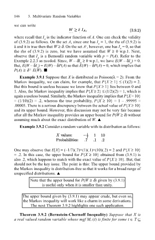
Example 3.9.2 Consider a random variable with its distribution as follows:

One may observe that E[X] = (–1/7)(.7)+(1)(.1)+(10)(.2) = 2 and P{X ≥ 10}
= .2. In this case, the upper bound for P{X ≥ 10} obtained from (3.9.1) is
also .2, which happens to match with the exact value of P{X ≥ 10}. But, that
should not be the key issue. The point is this: The upper bound provided by
the Markov inequality is distribution-free so that it works for a broad range of
unspecified distributions. !
Note that the upper bound for P(W ≥ δ) given by (3.9.1)
is useful only when it is smaller than unity.

The upper bound given by (3.9.1) may appear crude, but even so,
the Markov inequality will work like a charm in some derivations.
The next Theorem 3.9.2 highlights one such application.

Theorem 3.9.2 (Bernstein-Chernoff Inequality) Suppose that X is
a real valued random variable whose mgf Mx (t) is finite for some t ∈ T ⊆