Page 170 - Probability and Statistical Inference

3. Multivariate Random Variables 147

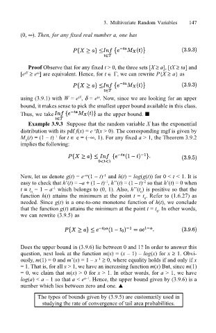
(0, ∞). Then, for any fixed real number a, one has

Proof Observe that for any fixed t > 0, the three sets [X ≥ a], [tX ≥ ta] and
tX
ta
[e ≥ e ] are equivalent. Hence, for t ∈ Γ, we can rewrite P{X ≥ a} as

using (3.9.1) with W = e , δ = e . Now, since we are looking for an upper
tX
ta
bound, it makes sense to pick the smallest upper bound available in this class.
Thus, we take as the upper bound. ¢
Example 3.9.3 Suppose that the random variable X has the exponential
distribution with its pdf f(x) = e I(x > 0). The corresponding mgf is given by
–x
M (t) = (1 – t) for t ∈ e = (–∞, 1). For any fixed a > 1, the Theorem 3.9.2
–1
X
implies the following:

Now, let us denote g(t) = e (1 – t) and h(t) = log(g(t)) for 0 < t < 1. It is
–1
–ta
easy to check that h’(t) = –a + (1 – t) , h’’(t) = (1 – t) so that h’(t) = 0 when
–1
–2
–1
t ≡ t = 1 – a which belongs to (0, 1). Also, h’’(t ) is positive so that the
0
0
function h(t) attains the minimum at the point t = t . Refer to (1.6.27) as
0
needed. Since g(t) is a one-to-one monotone function of h(t), we conclude
that the function g(t) attains the minimum at the point t = t . In other words,
0
we can rewrite (3.9.5) as
Does the upper bound in (3.9.6) lie between 0 and 1? In order to answer this
question, next look at the function m(x) = (x – 1) – log(x) for x ≥ 1. Obvi-
ously, m(1) = 0 and m’(x) = 1 – x ≥ 0, where equality holds if and only if x
–1
= 1. That is, for all x > 1, we have an increasing function m(x) But, since m(1)
= 0, we claim that m(x) > 0 for x > 1. In other words, for a > 1, we have
a–1
log(a) < a – 1 so that a < e . Hence, the upper bound given by (3.9.6) is a
number which lies between zero and one. !
The types of bounds given by (3.9.5) are customarily used in
studying the rate of convergence of tail area probabilities.