Page 174 - Probability and Statistical Inference

3. Multivariate Random Variables 151

Earlier we had seen applications of this covariance inequality in proving
the parts (ii)-(iii) in the Theorem 3.4.2 where we had shown that |ρX ,X | ≤ 1
1
2
whereas |ρX ,X | = 1 if and only if X = a + bX w.p.1.
1 2 1 2
Example 3.9.5 (Examples 3.2.4, 3.2.5, 3.4.1 Continued) For the two ran-
dom variables on hand, recall that we had V(X ) = 6.4971 and V(X ) = .6825.
1
2
Thus, Cov (X , X ) ≤ (6.4971)(.6825) ≈ 4.4343. But, we knew that Cov(X ,
2
2
1
1
X ) = –0.2415. !
2
Example 3.9.6 (Example 3.4.3, 3.4.6 Continued) For the two random
variables on hand, recall that we had V(X ) = 3/80 and V(X ) = 19/320. Thus,
1
2
2
Cov (X , X ) ≤ (3/80)(19/320) = 57/25600 ≈ .00223. But, we had found ear-
2
1
lier that Cov(X , X ) = 3/160 ≈ .01875. !
1 2
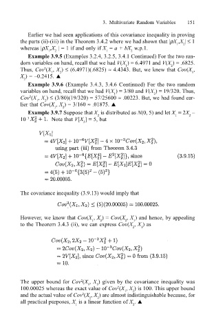
Example 3.9.7 Suppose that X is distributed as N(0, 5) and let X = 2X –
2
1
2
10 –3 Note that V[X ] = 5, but
2

The covariance inequality (3.9.13) would imply that

However, we know that Cov(X , X ) = Cov(X , X ) and hence, by appealing
2
2
1
1
to the Theorem 3.4.3 (ii), we can express Cov(X , X ) as
2 1

2
The upper bound for Cov (X , X ) given by the covariance inequality was
1
2
2
100.00025 whereas the exact value of Cov (X , X ) is 100. This upper bound
2
1
and the actual value of Cov (X , X ) are almost indistinguishable because, for
2
1 2
all practical purposes, X is a linear function of X . !
1 2