Page 178 - Probability and Statistical Inference

3. Multivariate Random Variables 155

Proof Note that if E[f(X)] is infinite, then the required inequality certainly
holds. So, let us assume now that E[f(X)] is finite. Since f(x) is convex, the
curve y = f(x) must lie above the tangents at all points (u, f(u)) for any u ∈ ℜ.
With u = E[X], consider specifically the point (u, f(u)) at which the equation
of the tangent line would be given by y = f(E[X]) + b{x – E[X]} for some
appropriate b. But, then we can claim that

Thus, using (3.9.21), we have
E[f(X)] = E[f(E(X)) + b{X – E(X)}] = f(E(X)) + b{E(X) – E(X)},
which reduces to f(E(X)). Thus, we have the desired result. ¢

In the statement of the Jensen’s inequality (3.9.20), equality
holds only when f(x) is linear in x ∈ ℜ. Also, the inequality
in (3.9.20) gets reversed when f(x) is concave.

Example 3.9.10 Suppose that X is distributed as Poisson (λ), λ > 0. Then,
3
using the Jensen’s inequality, for example, we immediately claim that E[X ] >
3
λ . This result follows because the function f(x) = x , x ∈ ℜ is convex and
+
3
E[X] = λ. !
Example 3.9.11 Suppose that X is distributed as N(–1, σ ), σ > 0. Then,
2
for example, we have E[|X|] > 1. This result follows immediately from the
Jensen’s inequality because the function f(x) = |x|, x ∈ ℜ is convex and |E[X]|
= |–1| = 1. !
2
Example 3.9.12 Suppose that X is distributed as N(µ, σ ), – ∞ < µ < ∞,
4
σ > 0. Then, for example, we have E[(X – µ) ] ≥ {E[(X – µ) ]} , by the
2
2
2
Jensen’s inequality with f(x) = x , x ∈ ℜ so that one can claim E[(X – µ) ]
4
+
4
2 2
≥ (σ ) = σ . !
Example 3.9.13 Suppose that one is proctoring a makeup examination for
two students who got started at the same time. Let X be the time to complete
i
the examination for the ith student, i = 1, 2. Let X = max (X , X ), the duration
1
2
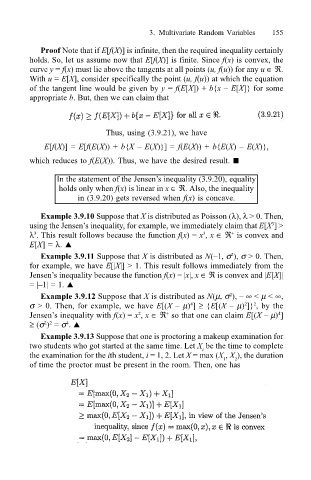
of time the proctor must be present in the room. Then, one has