Page 182 - Probability and Statistical Inference

3. Multivariate Random Variables 159

even though we may not know the exact distribution of , , k = 1, 2, ... .
2ξ
The following result actually gives an upper bound for E[| – µ | ] with
ξ ≥ 1/2.
Theorem 3.9.11 (Central Absolute Moment Inequality) Suppose that
we have iid real valued random variables X , X , ... having the common mean
1
2
2ξ
µ. Let us also assume that E[| X | ] < ∞ for some ξ ≥ 1/2. Then, we have
1
gwhere k does not depend on n, and T = 2ξ – 1 or ξ according as 1/2 ≤ ξ < 1
or ξ ≥ 1 respectively.
The methods for exact computations of central moments for the sample
mean were systematically developed by Fisher (1928). The classic text-
book of Cramér (1946a) pursued analogous techniques extensively. The par-
ticular inequality stated here is the special case of a more general large devia-
tion inequality obtained by Grams and Serfling (1973) and Sen and Ghosh
(1981) in the case of Hoeffding’s (1948) U-statistics. A sample mean turns
out to be one of the simplest U-statistics.

3.10 Exercises and Complements

3.2.1 (Example 3.2.2 Continued) Evaluate f (i) for i = –1, 0, 1.
2
3.2.2 (Example 3.2.4 Continued) Evaluate E[X | X = x ] where x = 1, 2.
1 2 2 2
3.2.3 (Example 3.2.5 Continued) Check that = 16.21. Also
evaluate
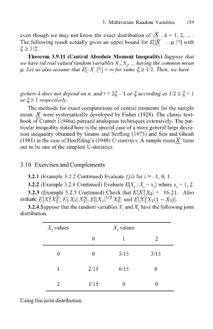
3.2.4 Suppose that the random variables X and X have the following joint
distribution. 1 2

X values X values
2 1
0 1 2

0 0 3/15 3/15

1 2/15 6/15 0

2 1/15 0 0

Using this joint distribution.