Page 181 - Probability and Statistical Inference

158 3. Multivariate Random Variables

3.9.7 Central Absolute Moment Inequality
Let X be a real valued random variable from some population having its pmf
or pdf f(x). Suppose that E[X], that is the population mean, is µ. In statistics,
th
k
E[| X – µ | ] is customarily called the k central absolute moment of X, k = 1,
2, ... . For example, suppose that X has the following distribution:
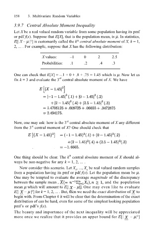
X values: –1 0 2 2.5
Probabilities: .1 .2 .4 .3

One can check that E[X] = –.1 + 0 + .8 + .75 = 1.45 which is µ. Now let us
rd
fix k = 3 and evaluate the 3 central absolute moment of X. We have

rd
Now, one may ask: how is the 3 central absolute moment of X any different
rd
from the 3 central moment of X? One should check that

th
One thing should be clear. The k central absolute moment of X should al-
ways be non-negative for any k = 1, 2, ... .
Now consider this scenario. Let X , ..., X be real valued random samples
1
n
from a population having its pmf or pdf f(x). Let the population mean be µ.
One may be tempted to evaluate the average magnitude of the discrepancy
between the sample mean , and the population
mean µ which will amount to E[| – µ|]. One may even like to evaluate
k
E[| – µ | ] for k = 1, 2, ... . But, then we need the exact distribution of to
begin with. From Chapter 4 it will be clear that the determination of the exact
distribution of can be hard, even for some of the simplest looking population
pmf’s or pdf’s f(x).
The beauty and importance of the next inequality will be appreciated
k
more once we realize that it provides an upper bound for E[| – µ| ]