Page 160 - Probability and Statistical Inference

3. Multivariate Random Variables 137

Hence, we can express ∫ ∫ g(x , x ; ρ) dx dx as
ℜ
2
1
1
2
2

Also, g(x , x ;ρ) is non-negative for all (x , x ) ∈ ℜ . Thus, g(x , x ) is a
2
2
1
1
2
1
2
genuine pdf on the support ℜ .
2
Let (X , X ) be the random variables whose joint pdf is g(x , x ;ρ) for all
1
2
2
1
(x , x ) ∈ ℜ . By direct integration, one can verify that marginally, both X and
2
2
1
1
X are indeed distributed as the standard normal variables.
2
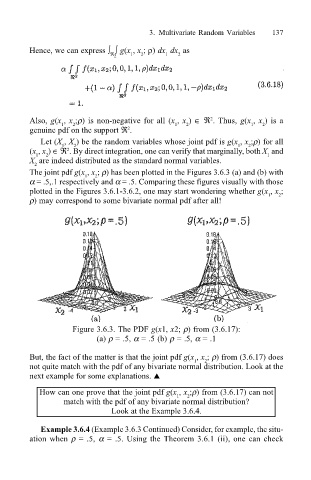
The joint pdf g(x , x ; ρ) has been plotted in the Figures 3.6.3 (a) and (b) with
2
1
α = .5,.1 respectively and α = .5. Comparing these figures visually with those
plotted in the Figures 3.6.1-3.6.2, one may start wondering whether g(x , x ;
2
1
ρ) may correspond to some bivariate normal pdf after all!

Figure 3.6.3. The PDF g(x1, x2; ρ) from (3.6.17):
(a) ρ = .5, α = .5 (b) ρ = .5, α = .1

But, the fact of the matter is that the joint pdf g(x , x ; ρ) from (3.6.17) does
1
2
not quite match with the pdf of any bivariate normal distribution. Look at the
next example for some explanations. !
How can one prove that the joint pdf g(x , x ;ρ) from (3.6.17) can not
2
1
match with the pdf of any bivariate normal distribution?
Look at the Example 3.6.4.
Example 3.6.4 (Example 3.6.3 Continued) Consider, for example, the situ-
ation when ρ = .5, α = .5. Using the Theorem 3.6.1 (ii), one can check