Page 366 - Probability and Statistical Inference

7. Point Estimation 343

from anthropometry and astronomy. The method of moments was introduced
by Pearson (1902).
The methodology is very simple. Suppose that θθ θθ θ = (θ , ..., θ ). Derive the
k
1
first k theoretical moments of the distribution f(x; θθ θθ θ) and pretend that they are
equal to the corresponding sample moments, thereby obtaining k equations in
k unknown parameters θ , ..., θ . Next, simultaneously solve these k equa-
k
1
tions for θ , ..., θ . The solutions are then the estimators of ? , ..., ? . Refer
1
k
1
k
back to the Section 2.3 as needed. To be more specific, we proceed as fol-
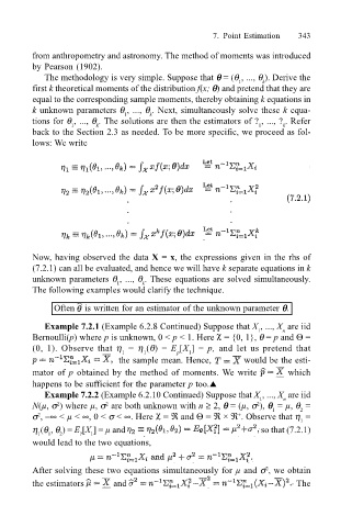
lows: We write

Now, having observed the data X = x, the expressions given in the rhs of
(7.2.1) can all be evaluated, and hence we will have k separate equations in k
unknown parameters θ , ..., θ . These equations are solved simultaneously.
k
1
The following examples would clarify the technique.

Often is written for an estimator of the unknown parameter θθ θθ θ.
Example 7.2.1 (Example 6.2.8 Continued) Suppose that X , ..., X are iid
n
1
χ
Bernoulli(p) where p is unknown, 0 < p < 1. Here = {0, 1}, θ = p and Θ =
(0, 1). Observe that η = η (θ) = E [X ] = p, and let us pretend that
1 1 p 1
the sample mean. Hence, would be the esti-
mator of p obtained by the method of moments. We write which
happens to be sufficient for the parameter p too.!
Example 7.2.2 (Example 6.2.10 Continued) Suppose that X , ..., X are iid
n
1
2
N(µ, σ ) where µ, σ are both unknown with n ≥ 2, θθ θθ θ = (µ, σ ), θθ θθ θ = µ, θ =
2
2
2
1
χ
σ , −∞ < µ < ∞, 0 < σ < ∞. Here = ℜ and Θ = ℜ × ℜ . Observe that η =
+
2
1
η (θ , θ ) = E [X ] = µ and so that (7.2.1)
1 1 2 ? 1
would lead to the two equations,
After solving these two equations simultaneously for µ and σ , we obtain
2
the estimators and . The