Page 370 - Probability and Statistical Inference

7. Point Estimation 347

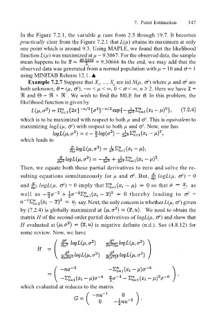
In the Figure 7.2.1, the variable µ runs from 2.5 through 19.7. It becomes
practically clear from the Figure 7.2.1 that L(µ) attains its maximum at only
one point which is around 9.3. Using MAPLE, we found that the likelihood
function L(µ) was maximized at µ = 9.3067. For the observed data, the sample
mean happens to be = 9.30666 In the end, we may add that the
observed data was generated from a normal population with µ = 10 and σ = 1
using MINITAB Release 12.1. !
2
Example 7.2.7 Suppose that X , ..., X are iid N(µ, σ ) where µ and σ are
2
1
n
both unknown, θ = (µ, σ ), −∞ < µ < ∞, 0 < σ < ∞, n ≥ 2. Here we have χ =
2
ℜ and Θ = ℜ × ℜ . We wish to find the MLE for θ. In this problem, the
+
likelihood function is given by
which is to be maximized with respect to both µ and σ . This is equivalent to
2
maximizing logL(µ, σ ) with respect to both µ and σ . Now, one has
2
2
which leads to

Then, we equate both these partial derivatives to zero and solve the re-
sulting equations simultaneously for µ and σ . But, logL(µ, σ ) = 0
2
2
and 2 logL(µ, σ ) = 0 imply that so that as
2
well as thereby leading to σ =
2
say. Next, the only concern is whether L(µ, σ ) given
2
by (7.2.4) is globally maximized at We need to obtain the
matrix H of the second-order partial derivatives of logL(µ, σ ) and show that
2
H evaluated at is negative definite (n.d.). See (4.8.12) for
some review. Now, we have

which evaluated at reduces to the matrix