Page 433 - Probability and Statistical Inference

410 8. Tests of Hypotheses

n = 2, 5, 6 and δ* = 2, 3. Express the critical region explicitly. !

In a discrete case, one applies the Neyman-Pearson Lemma, but
employs randomization. Look at Examples 8.3.6-8.3.7.

In all the examples, we have so far dealt with continuous distributions only.
The reader should recall the Remark 8.3.2. If the X’s are discrete, then we
carefully use randomization whenever L(x; θ ) = kL(x; θ ). The next two
0
1
examples emphasize this concept.
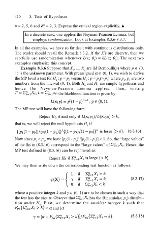
Example 8.3.6 Suppose that X , ..., X are iid Bernoulli(p) where p ∈ (0,
n
1
1) is the unknown parameter. With preassigned α ∈ (0, 1), we wish to derive
the MP level a test for H : p = p versus H : p = p (> p ) where p , p are two
0
0
1
0
1
0
1
numbers from the interval (0, 1). Both H and H are simple hypothesis and
0
1
hence the Neyman-Pearson Lemma applies. Then, writing
the likelihood function is given by
The MP test will have the following form:
that is, we will reject the null hypothesis H if
0
Now since p > p , we have [p (1 - p )]/[p (1 - p )] > 1. So, the “large values”
1 0 1 0 0 1
of the lhs in (8.3.16) correspond to the “large values” of Hence, the
MP test defined in (8.3.16) can be rephrased as:

We may then write down the corresponding test function as follows:

where a positive integer k and γ ∈ (0, 1) are to be chosen in such a way that
the test has the size α. Observe that has the Binomial(n, p ) distribu-
0
tion under H . First, we determine the smallest integer k such that
0
< α and let