Page 429 - Probability and Statistical Inference

406 8. Tests of Hypotheses

Since both H , H are simple hypotheses, the Neyman-Pearson Lemma
1
0
applies. The equation (8.3.6) will continue to hold but we now have µ – µ <
0
1
0. Thus the large values of will correspond to the
small values of . In other words, the MP test would look like
this:

This simplifies to the following form of the MP level a test:

See the Figure 8.3.2. Since E [X] = µ, it does make sense to reject H when
µ
0
is small because the alternative hypothesis postulates a value µ which is
1
smaller than µ . Under H , again observe that is a statistic,
0 0
referred to as the test statistic, which has a standard normal distribution.
Here, the critical region
– z .
α

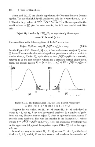
Figure 8.3.3. The Shaded Area is a, the Type I Error Probability:
(a) R ≡ {t ∈ T : t > k} (b) R ≡ {t ∈ T : t < k}
Suppose that we wish to test H : θ = θ versus H : θ = θ at the level α
0
0
1
1
where θ > θ and θ , θ are two known real numbers. In a number of prob-
1 0 0 1
lems, we may discover that we reject H when an appropriate test statistic T
0
exceeds some number k. This was the situation in the Example 8.3.1 where
we had and k = z . Here, the alternative hypothesis was
α
on the upper side (of µ ) and the rejection region R (for H ) fell on the upper
0
0
side too.
Instead we may wish to test H : θ = θ versus H : θ = θ at the level
1
1
0
0
α where θ < θ and θ , θ are two known real numbers. In a number of
1 0 0 1