Page 432 - Probability and Statistical Inference

8. Tests of Hypotheses 409

1/n
provided that we choose k = θ (1 – α) and implement test defined by
0
(8.3.13). Here, the critical region R = {X = (x , ..., x ) ∈ ℜ : x > θ (1 –
+n
1
n:n
0
n
α) }.
1/n
In the Neyman-Pearson Lemma, we assumed that θ was real valued.
This assumption was not crucial. The unknown parameter can be
vector valued too. It is crucial that the likelihood function involves
no unknown component of ? under either hypothesis H , i = 0, 1
i
if θ is vector valued. Look at Example 8.3.5.
Example 8.3.5 Suppose that X , ..., X are iid having the common pdf
n
1
b [G(δ)] x exp(–x/b) with two unknown parameters (δ, b) ∈ ℜ × ℜ , x ∈
-δ
+
δ-1
-1
+
ℜ . With preassigned α ∈ (0, 1), we wish to obtain the MP level α test for H 0
+
: (b = b , δ = δ*) versus H : (b = b , δ = δ*) where b > b are two positive
1
1
1
0
0
numbers and δ* is also a positive number. Both H and H are simple hypoth-
0
1
esis and hence the Neyman-Pearson Lemma applies. The likelihood function
is given by
The MP test will have the following form:
that is, we will reject the null hypothesis H if and only if
0
This test must also have size a. Observe that, under H , the statistic 3
0
has the Gamma (nδ*, b ) distribution which is completely known for fixed
0
values of n, δ*, b and α. Let us equivalently write the test as follows:
0
where g n,δ* , b is the upper 100a% point of the Gamma(nδ*, b ) distribution.
0
0,a
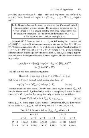
In the Table 8.3.1, g , b values are given for α = .01, .05, b = 1,
n,δ* 0,a 0
Table 8.3.1. Selected Values of g , b with b = 1
nδ* 0,α 0
α = .05 α = .01
n = 2 n = 5 n = 6 n = 2 n = 5 n = 6
δ* = 2 1.3663 5.4254 6.9242 0.8234 4.1302 5.4282
δ* = 3 2.6130 9.2463 11.6340 1.7853 7.4767 9.6163