Page 426 - Probability and Statistical Inference
P. 426
8. Tests of Hypotheses 403
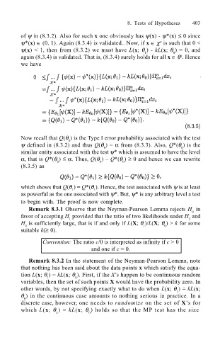
of ψ in (8.3.2). Also for such x one obviously has ψ(x) - ψ*(x) ≤ 0 since
ψ*(x) ∈ (0, 1). Again (8.3.4) is validated.. Now, if x ∈ χ is such that 0 <
n
ψ(x) < 1, then from (8.3.2) we must have L(x; θ ) - kL(x; θ ) = 0, and
1
0
again (8.3.4) is validated. That is, (8.3.4) surely holds for all x ∈ θ . Hence
n
we have
Now recall that Q(θ ) is the Type I error probability associated with the test
0
ψ defined in (8.3.2) and thus Q(θ ) = α from (8.3.3). Also, Q*(θ ) is the
0
0
similar entity associated with the test ψ* which is assumed to have the level
α, that is Q*(θ ) ≤ α. Thus, Q(θ ) Q*(θ ) ≥ 0 and hence we can rewrite
0
0
0
(8.3.5) as
which shows that Q(θ ) = Q*(θ ). Hence, the test associated with ψ is at least
1
1
as powerful as the one associated with ψ*. But, ψ* is any arbitrary level a test
to begin with. The proof is now complete.¾
Remark 8.3.1 Observe that the Neyman-Pearson Lemma rejects H in
0
favor of accepting H provided that the ratio of two likelihoods under H and
1
1
H is sufficiently large, that is if and only if L(X; θ )/L(X; θ ) > k for some
1
0
0
suitable k(≥ 0).
Convention: The ratio c/0 is interpreted as infinity if c > 0
and one if c = 0.
Remark 8.3.2 In the statement of the Neyman-Pearson Lemma, note
that nothing has been said about the data points x which satisfy the equa-
tion L(x; θ ) = kL(x; θ ). First, if the Xs happen to be continuous random
1
0
variables, then the set of such points X would have the probability zero. In
other words, by not specifying exactly what to do when L(x; θ ) = kL(x;
1
θ ) in the continuous case amounts to nothing serious in practice. In a
0
discrete case, however, one needs to randomize on the set of Xs for
which L(x; θ ) = kL(x; θ ) holds so that the MP test has the size
1 0

