Page 421 - Probability and Statistical Inference

398 8. Tests of Hypotheses

where R denotes a generic rejection region for H .
0
Example 8.2.2 (Example 8.2.1 Continued) In the case of the Test #1,
writing Z for a standard normal variable, we have:

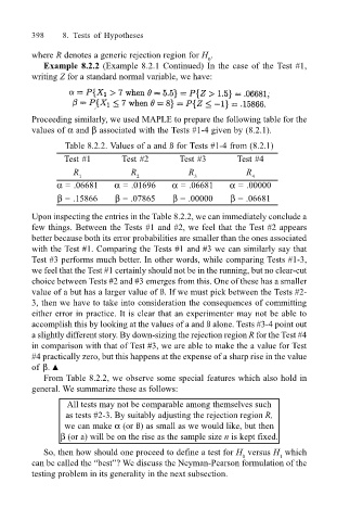
Proceeding similarly, we used MAPLE to prepare the following table for the
values of α and β associated with the Tests #1-4 given by (8.2.1).
Table 8.2.2. Values of a and ß for Tests #1-4 from (8.2.1)
Test #1 Test #2 Test #3 Test #4
R R R R
1 2 3 4
α = .06681 α = .01696 α = .06681 α = .00000
β = .15866 β = .07865 β = .00000 β = .06681
Upon inspecting the entries in the Table 8.2.2, we can immediately conclude a
few things. Between the Tests #1 and #2, we feel that the Test #2 appears
better because both its error probabilities are smaller than the ones associated
with the Test #1. Comparing the Tests #1 and #3 we can similarly say that
Test #3 performs much better. In other words, while comparing Tests #1-3,
we feel that the Test #1 certainly should not be in the running, but no clear-cut
choice between Tests #2 and #3 emerges from this. One of these has a smaller
value of a but has a larger value of ß. If we must pick between the Tests #2-
3, then we have to take into consideration the consequences of committing
either error in practice. It is clear that an experimenter may not be able to
accomplish this by looking at the values of a and ß alone. Tests #3-4 point out
a slightly different story. By down-sizing the rejection region R for the Test #4
in comparison with that of Test #3, we are able to make the a value for Test
#4 practically zero, but this happens at the expense of a sharp rise in the value
of β. !
From Table 8.2.2, we observe some special features which also hold in
general. We summarize these as follows:
All tests may not be comparable among themselves such
as tests #2-3. By suitably adjusting the rejection region R,
we can make α (or ß) as small as we would like, but then
β (or a) will be on the rise as the sample size n is kept fixed.
So, then how should one proceed to define a test for H versus H which
0
1
can be called the “best”? We discuss the Neyman-Pearson formulation of the
testing problem in its generality in the next subsection.