Page 552 - Probability and Statistical Inference

11. Likehood Ratio and Other Tests 529

the lines of (11.4.13), we can propose the following lower-sided level α test.

Two-Sided Alternative Hypothesis

We test H : σ = σ versus H : σ ≠ σ . See the Figure 11.4.4. Along the
1
2
1
0
1
2
lines of (11.4.11), we can propose the following two-sided level α test.
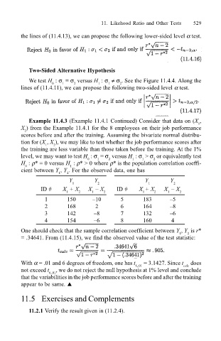
Example 11.4.3 (Example 11.4.1 Continued) Consider that data on (X ,
1
X ) from the Example 11.4.1 for the 8 employees on their job performance
2
scores before and after the training. Assuming the bivariate normal distribu-
tion for (X , X ), we may like to test whether the job performance scores after
1
2
the training are less variable than those taken before the training. At the 1%
level, we may want to test H : σ = σ versus H : σ > σ or equivalently test
1
0
2
1
2
1
H : ρ* = 0 versus H : ρ* > 0 where ρ* is the population correlation coeffi-
0 1
cient between Y , Y . For the observed data, one has
1 2
Y Y Y Y
1 2 1 2
ID # X + X X – X ID # X + X X – X
1 2 1 2 1 2 1 2
1 150 –10 5 183 –5
2 168 2 6 164 –8
3 142 –8 7 132 –6
4 154 –6 8 160 4
One should check that the sample correlation coefficient between Y , Y is r*
1
2
= .34641. From (11.4.15), we find the observed value of the test statistic:
With α = .01 and 6 degrees of freedom, one has t 6,.01 = 3.1427. Since t does
calc
not exceed t 6,.01 , we do not reject the null hypothesis at 1% level and conclude
that the variabilities in the job performance scores before and after the training
appear to be same. !

11.5 Exercises and Complements

11.2.1 Verify the result given in (11.2.4).