Page 547 - Probability and Statistical Inference

524 11. Likehood Ratio and Other Tests

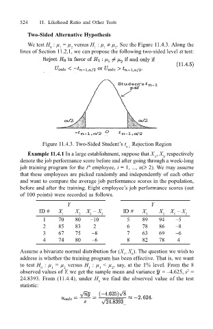
Two-Sided Alternative Hypothesis
We test H : µ = µ versus H : µ ≠ µ . See the Figure 11.4.3. Along the
1
1
2
2
0
1
lines of Section 11.2.1, we can propose the following two-sided level α test:

Figure 11.4.3. Two-Sided Student’s t Rejection Region
n-1
Example 11.4.1 In a large establishment, suppose that X , X respectively
1i
2i
denote the job performance score before and after going through a week-long
job training program for the i employee, i = 1, ..., n(≥ 2). We may assume
th
that these employees are picked randomly and independently of each other
and want to compare the average job performance scores in the population,
before and after the training. Eight employee’s job performance scores (out
of 100 points) were recorded as follows.
Y Y
ID # X X X – X ID # X X X – X
1 2 1 2 1 2 1 2
1 70 80 –10 5 89 94 –5
2 85 83 2 6 78 86 –8
3 67 75 –8 7 63 69 –6
4 74 80 –6 8 82 78 4

Assume a bivariate normal distribution for (X , X ). The question we wish to
1
2
address is whether the training program has been effective. That is, we want
to test H : µ = µ versus H : µ < µ , say, at the 1% level. From the 8
2
1
0
1
1
2
observed values of Y, we get the sample mean and variance = –4.625, s =
2
24.8393. From (11.4.4), under H we find the observed value of the test
0
statistic: