Page 189 - Process Modelling and Simulation With Finite Element Methods

176 Process Modelling and Simulation with Finite Element Methods

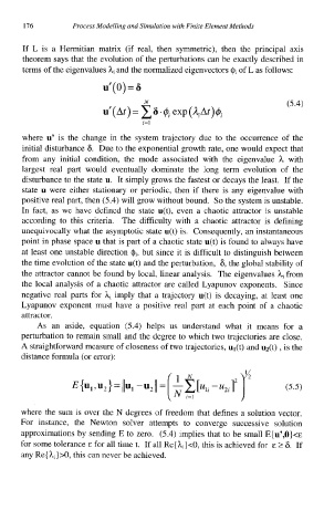
If L is a Hermitian matrix (if real, then symmetric), then the principal axis
theorem says that the evolution of the perturbations can be exactly described in
terms of the eigenvalues hi and the normalized eigenvectors Qi of L as follows:
u’(0) = 6

where u’ is the change in the system trajectory due to the occurrence of the
initial disturbance 6. Due to the exponential growth rate, one would expect that
from any initial condition, the mode associated with the eigenvalue h with
largest real part would eventually dominate the long term evolution of the
disturbance to the state u. It simply grows the fastest or decays the least. If the
state u were either stationary or periodic, then if there is any eigenvalue with
positive real part, then (5.4) will grow without bound. So the system is unstable.
In fact, as we have defined the state u(t), even a chaotic attractor is unstable
according to this criteria. The difficulty with a chaotic attractor is defining
unequivocally what the asymptotic state u(t) is. Consequently, an instantaneous
point in phase space u that is part of a chaotic state u(t) is found to always have
at least one unstable direction $, but since it is difficult to distinguish between
the time evolution of the state u(t) and the perturbation, 6, the global stability of
the attractor cannot be found by local, linear analysis. The eigenvalues hi from
the local analysis of a chaotic attractor are called Lyapunov exponents. Since
negative real parts for hi imply that a trajectory u(t) is decaying, at least one
Lyapunov exponent must have a positive real part at each point of a chaotic
attractor.
As an aside, equation (5.4) helps us understand what it means for a
perturbation to remain small and the degree to which two trajectories are close.
A straightforward measure of closeness of two trajectories, ul(t) and uz(t) , is the
distance formula (or error):

where the sum is over the N degrees of freedom that defines a solution vector.
For instance, the Newton solver attempts to converge successive solution
approximations by sending E to zero. (5.4) implies that to be small E{U’,O}<E
for some tolerance E for all time t. If all Re{ hi}<O, this is achieved for E 2 6. If
any Re{hi}>O, this can never be achieved.