Page 208 - Process Modelling and Simulation With Finite Element Methods

Simulation and Nonlinear Dynamics 195

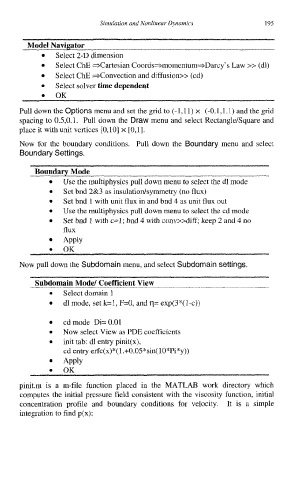
Select ChE +Cartesian Coordsqmomentum3Darcy's Law >> (dl)
Select ChE d2onvection and diffusion>> (cd)
Select solver time dependent

Pull down the Options menu and set the grid to (-1,ll) x (-0. I, 1.1) and the grid
spacing to 0.5,O.l. Pull down the Draw menu and select RectangleBquare and
place it with unit vertices [0,10] x [0,1].
Now for the boundary conditions. Pull down the Boundary menu and select
Boundary Settings.

Boundary Mode
Use the multiphysics pull down menu to select the dl mode
Set bnd 2&3 as insulatiodsymmetry (no flux)
Set bnd 1 with unit flux in and bnd 4 as unit flux out
Use the multiphysics pull down menu to select the cd mode
Set bnd 1 with c=l; bnd 4 with conv>>diff; keep 2 and 4 no
flux
APPlY

Now pull down the Subdomain menu, and select Subdomain settings.
Subdomain Mode/ Coefficient View
Select domain 1
0
dl mode, set k=l, F=O, and q= exp(3 *( 1 -c))

cdmode Di=0.01
0 Now select View as PDE coefficients
0 init tab: dl entry pinit(x),
cd entry erfc(x)*( 1 .+0.05*sin( 10*Pi*y))
APPlY
OK

pinit.m is a m-file function placed in the MATLAB work directory which
computes the initial pressure field consistent with the viscosity function, initial
concentration profile and boundary conditions for velocity. It is a simple
integration to find p(x):