Page 214 - Process Modelling and Simulation With Finite Element Methods

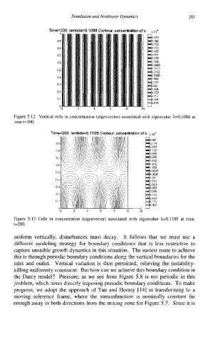
Simulation and Nonlinear Dynamics 201

Time=200 lambda=0.1088 Contour: concentration of c . ,,4
1
6 019
09 5 386
4 752
08 4 119
3 485
07 2 851
2 218
06 1 584
0 9508
05 03173
0 3163
0 9498
04
1 583
2 217
03 2 85
3 484
02 4 118
4 751
01 5 385
6 018
0
2 4 6 8 10
Figure 5.12 Vertical rolls in concentration (eigenvector) associated with eigenvalue h=0.1088 at
time t=200.
Time=200 lambda=0.1108 Contour: concentration of c
103
6 901
6 174
5 448
4 722
3 995
3 269
2 542
1816
1 089
0 362g
0 3635
1 09
1816
2 543
3 269
3 996
4 722
5 443
6 116
6 902
12
Figure 5.13 Cells in concentration (eigenvector) associated with eigenvalue h=O. 1108 at time.
t=200.
uniform vertically, disturbances must decay. It follows that we must use a
different modeling strategy for boundary conditions that is less restrictive to
capture unstable growth dynamics in this situation. The easiest route to achieve
this is through periodic boundary conditions along the vertical boundaries for the
inlet and outlet. Vertical variation is then permitted, relieving the instability-
killing uniformity constraint. But how can we achieve this boundary condition in
the Darcy model? Pressure, as we see from Figure 5.8 is not periodic in this
problem, which nixes directly imposing periodic boundary conditions. To make
progress, we adopt the approach of Tan and Homsy [14] in transforming to a
moving reference frame, where the streamfunction is nominally constant far
enough away in both directions from the mixing zone for Figure 5.7. Since it is