Page 216 - Process Modelling and Simulation With Finite Element Methods

Simulation and Nonlinear Dynamics 203

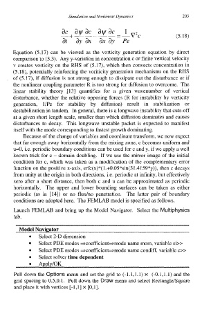
(5.18)

Equation (5.17) can be viewed as the vorticity generation equation by direct
comparison to (3.3). Any y-variation in concentration c or finite vertical velocity
v creates vorticity on the RHS of (5.17), which then convects concentration in
(5.18), potentially reinforcing the voriticity generation mechanisms on the RHS
of (5.17), if diffusion is not strong enough to dissipate out the disturbance or if
the nonlinear coupling parameter R is too strong for diffusion to overcome. The
linear stability theory [13] quantifies for a given wavenumber of vertical
disturbance, whether the relative opposing forces (R for instability by vorticity
generation, 1Pe for stability by diffusion) result in stabilization or
destabilization in tandem. In general, there is a longwave instability that cuts-off
at a given short length scale, smaller than which diffusion dominates and causes
disturbances to decay. This longwave unstable packet is expected to manifest
itself with the mode corresponding to fastest growth dominating.
Because of the change of variables and coordinate transform, we now expect
that far enough away horizontally from the mixing zone, c becomes uniform and
u=0, i.e. periodic boundary conditions can be used for c and y, if we apply a well
known trick for c - domain doubling. If we use the mirror image of the initial
condition for c, which was taken as a modification of the complementary error
function on the positive x-axis, erfc(x)*( 1 .+0.05*sin(3 1.4159*y)), then c decays
from unity at the origin in both directions, i.e. periodic at infinity, but effectively
zero after a short distance, then both c and u can be approximated as periodic
horizontally. The upper and lower bounding surfaces can be taken as either
periodic (as in [14]) or no fludno penetration. The latter pair of boundary
conditions are adopted here. The FEMLAB model is specified as follows.
Launch FEMLAB and bring up the Model Navigator. Select the Multiphysics
tab.
Model Navigator
Select 2-D dimension
Select PDE modes =xoefficient*mode name mom, variable si>>
Select PDE modes =xoefficient*mode name condiff, variable c>>
Select solver time dependent

Pull down the Options menu and set the grid to (-1.1,l.l) x (-0.1,l.l) and the
grid spacing to 0.5,O.l. Pull down the Draw menu and select Rectangle/Square
and place it with vertices [-1,1] x [0,1].