Page 221 - Process Modelling and Simulation With Finite Element Methods

208 Process Modelling and Simulation with Finite Element Methods

0.3854 0.4109 0.4837
0.4869 - 0.0131i
0.4869 + 0.0131i 0.5099
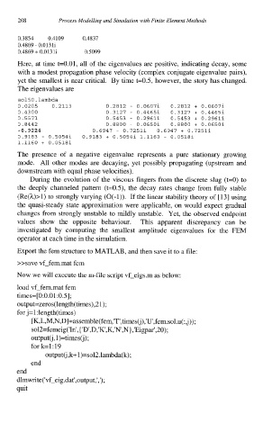
Here, at time t=0.01, all of the eigenvalues are positive, indicating decay, some
with a modest propagation phase velocity (complex conjugate eigenvalue pairs),
yet the smallest is near critical. By time t=0.5, however, the story has changed.
The eigenvalues are
so150.lambda
0.0205 0.2113 0.2812 - 0.0607i 0.2812 + 0.0607i
0.4300 0.3127 - 0.4465i 0.3127 + 0.4465i
0.5571 0.5453 - 0.2961i 0.5453 + 0.2961i
0.8442 0.8800 - 0.065Oi 0.8800 + 0.065Oi
-0.9224 0.6947 - 0.72511 0.6947 + 0.7251i
0.9183 - 0.5054i 0.9183 + 0.5054i 1.1160 - 0.0518i
1.1160 + 0.0518i
The presence of a negative eigenvalue represents a pure stationary growing
mode. All other modes are decaying, yet possibly propagating (upstream and
downstream with equal phase velocities).
During the evolution of the viscous fingers from the discrete slug (t=O) to
the deeply channeled pattern (t=0.5), the decay rates change from fully stable
(Re(h)>l) to strongly varying (O(-1)). If the linear stability theory of [13] using
the quasi-steady state approximation were applicable, on would expect gradual
changes from strongly unstable to mildly unstable. Yet, the observed endpoint
values show the opposite behaviour. This apparent discrepancy can be
investigated by computing the smallest amplitude eigenvalues for the FEM
operator at each time in the simulation.
Export the fem structure to MATLAB, and then save it to a file:
>>save vf-fem.mat fem
Now we will execute the m-file script vf-eigs.m as below:
load vf-fem.mat fem
times=[0:0.01:0.5];
output=zeros(length(times),2 1);
for j=l:length(times)
[K,L,M,N,D]=assemble(fem,'T',times(j),'U,fem.sol.u(
:j));
sol2=femeig('In', { 'D',D,'K,K,'N,N} ,'Eigpar',20);
output(j, l)=times(j);
for k=1:19
output(j ,k+ l)=sol2,lambda(k);
end
end
dlmwrite('vf-eig.dat',output,',');
quit