Page 81 - Process Modelling and Simulation With Finite Element Methods

68 Process Modelling and Simulation with Finite Element Methods

, Streamfunctiwn
I I
................. ...........

a .............. .....

x .................... ...........

-0

I I I
-2 -1 5 .I -0 5 0 05 1 15
X
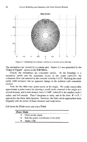
Figure 2.1 Streamlines for constant vorticity in a circular cavity with slip.

The streamlines are viewed by a contour plot. Figure 2.1 was generated by the
“Copy to Figure” option on the Edit Menu.
Clearly, the streamlines are concentric circles. As the boundary is a
streamline (ty=O) and the maximum occurs in the center (t+e0.25), the
volumetric flow rate induced by the constant vorticity is 0.25. Refining the mesh
yields 2480 elements, but no apparent change in the solution (still concentric
circles).
Now, for the other case: point source at the origin. We could conceivably
approximate a point source by drawing a small circle centered at the origin as a
second domain, and in that domain, have f=lhR2, where R is the smaller circle’s
radius, and f=O outside. Then f integrates to unity, and in the limit R + 0, f
approaches the Dirac delta function. However, the limit can be approached more
elegantly with the power of finite elements and weak terms.

Pull down the Draw menu and select Point.

Draw Mode
Click on the origin
Edit the points coordinates to be (0,O)
Apply/OK