Page 72 - Rapid Learning in Robotics

58 The PSOM Algorithm

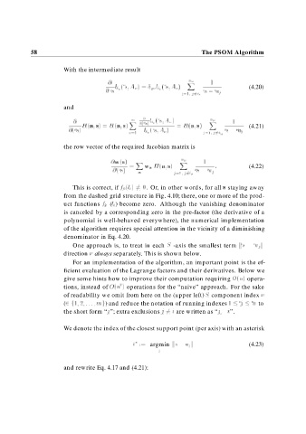
With the intermediate result

n

X

l i s A l i s A (4.20)

s s a j

j i j

and

n
l i s A
m

X
s X

H a s H a s H a s (4.21)

s l i s A s a j

j
i

j
the row vector of the required Jacobian matrix is
n

w s X X

w a H a s (4.22)

s a s a j

j
i

j
This is correct, if f k l i . Or, in other words, for all s staying away
from the dashed grid structure in Fig. 4.10; there, one or more of the prod-
uct functions f k (l i) become zero. Although the vanishing denominator
is canceled by a corresponding zero in the pre-factor (the derivative of a
polynomial is well-behaved everywhere), the numerical implementation
of the algorithm requires special attention in the vicinity of a diminishing
denominator in Eq. 4.20.
One approach is, to treat in each S -axis the smallest term ks a j k

direction always separately. This is shown below.
For an implementation of the algorithm, an important point is the ef-
ficient evaluation of the Lagrange factors and their derivatives. Below we
give some hints how to improve their computation requiring O n opera-

tions, instead of O n operations for the “naive” approach. For the sake
of readability we omit from here on the (upper left) S component index
m
(
g) and f reduce the notation of running indexes j n to

the short form “j”; extra exclusions j i are written as “j i”.
We denote the index of the closest support point (per axis) with an asterisk

i argmin ks a j k (4.23)
j
and rewrite Eq. 4.17 and (4.21):