Page 42 -

2.2 Linear State-Variable Systems 23

u(t)=α 1 u 1 (t)+α 2 u 2 (t) is given by y(t)=α 1 y 1 (t)+α 2 y 2 (t), where α 1 and α 2 are scalar
constants. Linear, single-input/single-output (SISO), continuous-time, time-
invariant systems are described by linear, scalar, constant-coefficient ordinary
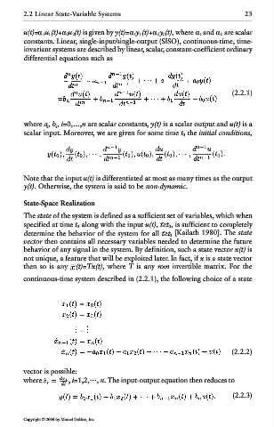
differential equations such as

(2.2.1)

where a i , b i , i=0,…,n are scalar constants, y(t) is a scalar output and u(t) is a
scalar input. Moreover, we are given for some time t 0 the initial conditions,

Note that the input u(t) is differentiated at most as many times as the output
y(t). Otherwise, the system is said to be non-dynamic.

State-Space Realization
The state of the system is defined as a sufficient set of variables, which when
specified at time t 0 along with the input u(t), t≥t 0 , is sufficient to completely
determine the behavior of the system for all t≥t 0 [Kailath 1980]. The state
vector then contains all necessary variables needed to determine the future
behavior of any signal in the system. By definition, such a state vector x(t) is
not unique, a feature that will be exploited later. In fact, if x is a state vector
then so is any (t)=Tx(t), where T is any n×n invertible matrix. For the
continuous-time system described in (2.2.1), the following choice of a state

(2.2.2)

vector is possible:
where , i=1,2, … , n. The input-output equation then reduces to

(2.2.3)

Copyright © 2004 by Marcel Dekker, Inc.