Page 43 -

24 Introduction to Control Theory

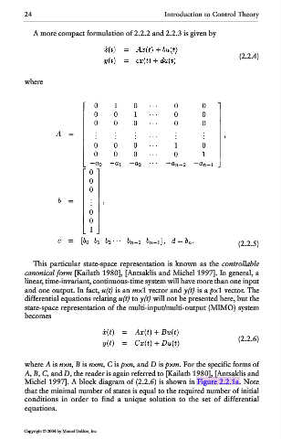
A more compact formulation of 2.2.2 and 2.2.3 is given by

(2.2.4)

where

(2.2.5)

This particular state-space representation is known as the controllable
canonical form [Kailath 1980], [Antsaklis and Michel 1997]. In general, a
linear, time-invariant, continuous-time system will have more than one input
and one output. In fact, u(t) is an m×1 vector and y(t) is a p×1 vector. The
differential equations relating u(t) to y(t) will not be presented here, but the
state-space representation of the multi-input/multi-output (MIMO) system
becomes

(2.2.6)

where A is n×n, B is n×m, C is p×n, and D is p×m. For the specific forms of
A, B, C, and D, the reader is again referred to [Kailath 1980], [Antsaklis and
Michel 1997]. A block diagram of (2.2.6) is shown in Figure 2.2.1a. Note
that the minimal number of states is equal to the required number of initial
conditions in order to find a unique solution to the set of differential
equations.

Copyright © 2004 by Marcel Dekker, Inc.