Page 108 - Robot Builders Source Book - Gordon McComb

3.5 Pneumodrive 97

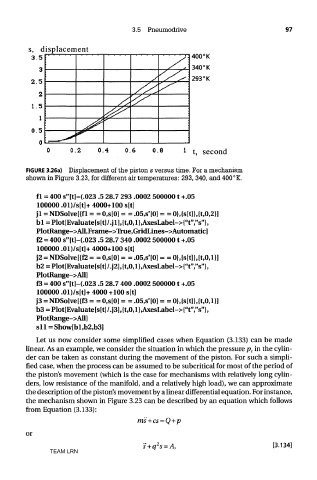
FIGURE 3.26a) Displacement of the piston s versus time. For a mechanism
shown in Figure 3.23, for different air temperatures: 293, 340, and 400°K.

fl = 400 s"[t]-(.023 .5 28.7 293 .0002 5000001 +.05
100000 .01)/s[t]+ 4000+100 s[t]
jl = NDSolve[{fl = = 0,s[0] = = .05,s'[0] = = 0},{s[t]},{t,0,2}]
bl = Plot[Evaluate[s[t]/.jl],{t,0,l},AxesLabel->{"t","s"},
PlotRange->All,Frame->True,GridLines->Automatic]
f2 = 400 s"[t]-(.023 .5 28.7 340 .0002 5000001 +.05
100000 .01)/s[t]+ 4000+100 s[t]
j2 = NDSolve[{f2= = 0,s[0] = =.05,s'[0] = =0},{s[t]},{t,0,l}]
b2 = Plot[Evaluate[s[t]/.j2],{t,0,l}^AxesLabel->{"t","s"},
PlotRange->All]
f3 = 400 s"[t]-(.023 .5 28.7 400 .0002 5000001 +.05
100000 .01)/s[t]+ 4000 +100 s[t]
j3 = NDSolve[{f3 = = 0,s[0] = = .05,s'[0] = = 0},{s[t]},{t,0,l}]
b3 = Plot[Evaluate[s[t]/.j3],{t,0,l} >AxesLabel->{"t","s"},
PlotRange->All]
sll = Show[bl,b2,b3]
Let us now consider some simplified cases when Equation (3.133) can be made
linear. As an example, we consider the situation in which the pressure p c in the cylin-
der can be taken as constant during the movement of the piston. For such a simpli-
fied case, when the process can be assumed to be subcritical for most of the period of
the piston's movement (which is the case for mechanisms with relatively long cylin-
ders, low resistance of the manifold, and a relatively high load), we can approximate
the description of the piston's movement by a linear differential equation. For instance,
the mechanism shown in Figure 3.23 can be described by an equation which follows
from Equation (3.133):

or

TEAM LRN