Page 101 - Robotics Designing the Mechanisms for Automated Machinery

90 Dynamic Analysis of Drives

Integrating this, latter expression we obtain the required formula in the following form:

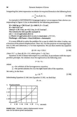
An example in MATHEMATICA language is given. Let us suppose that a device cor-
responding to Figure 3.22a) is described by the following parameters:
2
2
M = 1000 kg, p = 700 N/cm , Q = 5000 N, F = 75 cm ,
2 2
¥=100Nsec /m .
2
Then ft = 4.36 I/sec, m = 0.2 1/m, A = 47.5 ml sec .
The solution for this specific example is:
s[t] = = 2/.2 Log[Cosh[4.36/2 t]l
j = Plot[2/.2 Log[Cosh[4.36/2 t]],{t,0,.l},AxesLabel->{"t","s"},
PlotRange->AU,Frame->True,GridLines->Automaticl
It is more difficult to solve the problem for a case in which the value A varies, say,
a function of the piston's displacement. Thus: A(s). For this purpose we rearrange Equa-
2
tion (3.100) and substitute y = s in that expression. We can then rewrite the equation
in the form

2
(Note: If s = y, then dy/dt=2ss, which gives s = dy/2ds.}
Equation (3.105) is linear with respect to y, and thus, in accordance with the super-
position principle, the solution must be expressed as the following sum:

where
y 0 = the solution of the homogeneous equation,
y l = the partial solution for A in the right-hand side of the equation.
We seek y 0 in the form

Substituting Equation (3.106) into Equation (3.105), we find that

FIGURE 3.22a) Solution: piston displacement versus
time for the above-given mechanism.