Page 72 - Satellite Communications, Fourth Edition

52 Chapter Two

in terms of an intermediate variable E, known as the eccentric anom-
aly, and is usually stated as

M 5 E e sin E (2.27)

Kepler’s equation is derived in App. B. This rather innocent looking
equation is solved by iterative methods, usually by finding the root of
the equation:

M (E e sin E ) 5 0 (2.28)
The following example shows how to solve for E graphically.

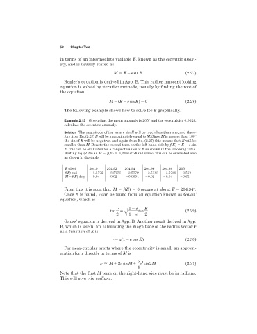
Example 2.13 Given that the mean anomaly is 205° and the eccentricity 0.0025,
calculate the eccentric anomaly.

Solution The magnitude of the term e sin E will be much less than one, and there-
fore from Eq. (2.27) E will be approximately equal to M. Since M is greater than 180°
the sin of E will be negative, and again from Eq. (2.27) this means that E will be
smaller than M. Denote the second term on the left-hand side by f(E) E e sin
E; this can be evaluated for a range of values of E as shown in the following table.
Writing Eq. (2.28) as M f(E ) 5 0 , the left-hand side of this can be evaluated also
as shown in the table.

E (deg) 204.9 204.92 204.94 204.96 204.98 205
f(E) rad 3.5772 3.5776 3.5779 3.5783 3.5786 3.579
M f(E) deg 0.04 0.02 0.0004 0.02 0.04 0.61

From this it is seen that M f(E ) 0 occurs at about E 204.94°.
Once E is found, can be found from an equation known as Gauss’
equation, which is

tan 5 1 e tan E (2.29)
2 B1 e 2
Gauss’ equation is derived in App. B. Another result derived in App.
B, which is useful for calculating the magnitude of the radius vector r
as a function of E is
r 5 a(1 e cos E ) (2.30)

For near-circular orbits where the eccentricity is small, an approxi-
mation for directly in terms of M is

5 2
v > M 2e sin M e sin 2M (2.31)
4
Note that the first M term on the right-hand side must be in radians.
This will give in radians.