Page 123 - Schaum's Outline of Theory and Problems of Signals and Systems

LAPLACE TRANSFORM AND CONTINUOUS-TIME LTI SYSTEMS [CHAP. 3

s-plane

(a) (b)
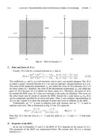
Fig. 3-1 ROC for Example 3.1.

C. Poles and Zeros of X( s 1:
Usually, X(s) will be a rational function in s, that is,

The coefficients a, and b, are real constants, and m and n are positive integers. The X(s)
is called a proper rational function if n > m, and an improper rational function if n I m.
The roots of the numerator polynomial, z,, are called the zeros of X(s) because X(s) = 0
for those values of s. Similarly, the roots of the denominator polynomial, p,, are called the
poles of X(s) because X(s) is infinite for those values of s. Therefore, the poles of X(s)
lie outside the ROC since X(s) does not converge at the poles, by definition. The zeros, on
the other hand, may lie inside or outside the ROC. Except for a scale factor ao/bo, X(s)
can be completely specified by its zeros and poles. Thus, a very compact representation of
X(s) in the s-plane is to show the locations of poles and zeros in addition to the ROC.
Traditionally, an " x " is used to indicate each pole location and an " 0 " is used to
indicate each zero. This is illustrated in Fig. 3-3 for X(s) given by

Note that X(s) has one zero at s = - 2 and two poles at s = - 1 and s = - 3 with scale
factor 2.

D. Properties of the ROC:
As we saw in Examples 3.1 and 3.2, the ROC of X(s) depends on the nature of dr).
The properties of the ROC are summarized below. We assume that X(s) is a rational
function of s.