Page 130 - Schaum's Outline of Theory and Problems of Signals and Systems

CHAP. 31 LAPLACE TRANSFORM AND CONTINUOUS-TIME LTI SYSTEMS

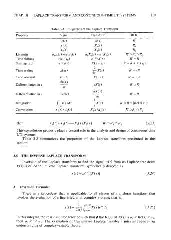
Table 3-2 Properties of the Laplace Transform
Property Signal Transform ROC

x(t) X(s) R
x,(t) x,w R 1
x2W x,w R2
Linearity a,x,(t) + a2x2(l) a, X,(s) + a, X2(s) R'IR, nR2
Time shifting x(t - to) e-""X(s) R' = R
Shifting in s es"'x( t X(s - so) R' = R + Re(s,)
1
Time scaling x( at -X(s) R' = aR
la l
Time reversal R'= -R

Differentiation in t
dX( s)
Differentiation in s - tx(t) Rf=R
ds

Integration
Convolution

then %(t) * ~20) HXI(~)X~(~) R'IR, nR2 (3.23)

This convolution property plays a central role in the analysis and design of continuous-time
LTI systems.
Table 3-2 summarizes the properties of the Laplace transform presented in this
section.

3.5 THE INVERSE LAPLACE TRANSFORM

Inversion of the Laplace transform to find the signal x(t) from its Laplace transform
X(s) is called the inverse Laplace transform, symbolically denoted as

A. Inversion Formula:

There is a procedure that is applicable to all classes of transform functions that
involves the evaluation of a line integral in complex s-plane; that is,

In this integral, the real c is to be selected such that if the ROC of X(s) is a, < Re(s) <a2,
then a, < c < u2. The evaluation of this inverse Laplace transform integral requires an
understanding of complex variable theory.