Page 132 - Schaum's Outline of Theory and Problems of Signals and Systems

CHAP. 31 LAPLACE TRANSFORM AND CONTINUOUS-TIME LTI SYSTEMS 121

is a polynomial in s with degree strictly less than n. The inverse Laplace transform of X(s)
can then be computed by determining the inverse Laplace transform of Q(s) and the
inverse Laplace transform of R(s)/D(s). Since R(s)/D(s) is proper, the inverse Laplace
transform of R(s)/D(s) can be computed by first expanding into partial fractions as given
above. The inverse Laplace transform of Q(s) can be computed by using the transform
pair

3.6 THE SYSTEM FUNCTION

A. The System Function:
In Sec. 2.2 we showed that the output y(t) of a continuous-time LTI system equals the
convolution of the input x(t) with the impulse response h(t); that is,

Applying the convolution property (3.23), we obtain

where Y(s), X(s), and H(s) are the Laplace transforms of y(t), x(t), and h(t), respec-
tively. Equation (3.36) can be expressed as

The Laplace transform H(s) of h(t) is referred to as the system function (or the transfer
function) of the system. By Eq. (3.37), the system function H(s) can also be defined as the
ratio of the Laplace transforms of the output y(t) and the input x(t). The system function
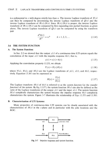
H(s) completely characterizes the system because the impulse response h(t) completely
characterizes the system. Figure 3-7 illustrates the relationship of Eqs. (3.35) and (3.36).

B. Characterization of LTI Systems:
Many properties of continuous-time LTI systems can be closely associated with the
characteristics of H(s) in the s-plane and in particular with the pole locations and the
ROC.

Fig. 3-7 Impulse response and system function.