Page 315 - Schaum's Outline of Theory and Problems of Signals and Systems

302 FOURIER ANALYSIS OF DISCRETE-TIME SIGNALS AND SYSTEMS [CHAP. 6

B. LTI Systems Characterized by Difference Equations:

As discussed in Sec. 2.9, many discrete-time LTI systems of practical interest are
described by linear constant-coefficient difference equations of the form
N M
C aky[n - k] = C b,x[n - k] (6.76)
k=O k=O
with MI N. Taking the Fourier transform of both sides of Eq. (6.76) and using the
linearity property (6.42) and the time-shifting property (6.43), we have
N M
C a, e-jkRY(R) = C bk e-Jkb'X
(a)
k=O k=O
or, equivalently,
M

The result (6.77) is the same as the 2-transform counterpart H(z) = Y(z)/X(z) with
z = eJ" [Eq. (4.4411; that is,

C. Periodic Nature of the Frequency Response:

From Eq. (6.41) we have
H(R) = H(n + 27r)
Thus, unlike the frequency response of continuous-time systems, that of all discrete-time
LTI systems is periodic with period 27r. Therefore, we need observe the frequency
response of a system only over the frequency range 0 I R R 27r or -7r I I R T.

6.6 SYSTEM RESPONSE TO SAMPLED CONTINUOUS-TIME SINUSOIDS
A. System Responses:

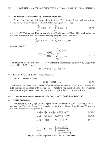
We denote by y,[n], y,[n], and y[n] the system responses to cos Rn, sin Rn, and eJRn,
respectively (Fig. 6-4). Since e~~'" = cos Rn + j sin Rn, it follows from Eq. (6.72) and the
linearity property of the system that
y [n] = y,[n] + jy,[n] = H(R) eJRn

~,[n]
= Re{y[n]) = R~(H(R) eJRn)
y,[n] = I~{Y [nl ) = Im{H(R)

Fig. 6-4 System responses to elnn, cos Rn, and sin Rn.