Page 352 - Schaum's Outline of Theory and Problems of Signals and Systems

CHAP. 61 FOURIER ANALYSIS OF DISCRETE-TIME SIGNALS AND SYSTEMS

From T, = 1,

For T, = 0.1,

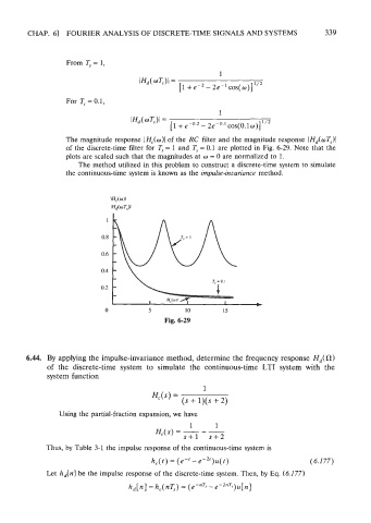
The magnitude response IHc(w)l of the RC filter and the magnitude response IH,(wq)l
of the discrete-time filter for T, = 1 and T, = 0.1 are plotted in Fig. 6-29. Note that the
plots are scaled such that the magnitudes at w = 0 are normalized to 1.
The method utilized in this problem to construct a discrete-time system to simulate
the continuous-time system is known as the impulse-inuariance method.

0 5 10 15
Fig. 6-29

6.44. By applying the impulse-invariance method, determine the frequency response Hd(fl)
of the discrete-time system to simulate the continuous-time LTI system with the
system function

Using the partial-fraction expansion, we have

Thus, by Table 3-1 the impulse response of the continuous-time system is

hc(t) = (e-t - e-")u(t) (6.177)
Let hd[nl be the impulse response of the discrete-time system. Then, by Eq. (6.177)
hd[n] = h,(nT,) = (e-"'5 - e-'"'j )4n]