Page 365 - Schaum's Outline of Theory and Problems of Signals and Systems

FOURIER ANALYSIS OF DISCRETE-TIME SIGNALS AND SYSTEMS [CHAP. 6

(N/2)- I
N
where F[kl = C f[nlW,k;2 k=O,l, ...,- - 1
2
n=O

Note that F[k] and G[k] are the (N/2)-point DFTs of fin] and gin], respectively. Now

Hence, Eq. (6.221) can be expressed as

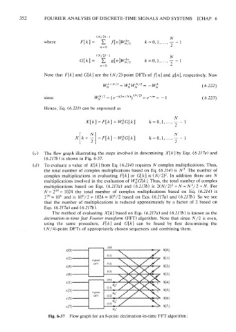
(c) The flow graph illustrating the steps involved in determining X[k] by Eqs. (6.217~) and
(6.21 76) is shown in Fig. 6-37.
(d) To evaluate a value of X[k] from Eq. (6.214) requires N complex multiplications. Thus,
the total number of complex multiplications based on Eq. (6.214) is N~. The number of
complex multiplications in evaluating F[k] or G[k] is (N/2)2. In addition there are N
multiplications involved in the evaluation of ~,k~[k]. Thus, the total number of complex
multiplications based on Eqs. (6.217~) and (6.217b) is 2(~/2)~ = ~'/2 + N. For
+ N
N = 2"'= 1024 the total number of complex multiplications based on Eq. (6.214) is
22" -- loh and is 106/2 + 1024 .= 106/2 based on Eqs. (6.217~) and (6.217b). So we see
that the number of multiplications is reduced approximately by a factor of 2 based on
Eqs. (6.217~) and (6.2176).
The method of evaluating X[k I based on Eqs. (6.217~) and (6.217b) is known as the
decimation-in-time fast Fourier transform (FFT) algorithm. Note that since N/2 is even,
using the same procedure, F[kl and G[k] can be found by first determining the
(N/4)-point DFTs of appropriately chosen sequences and combining them.

Fig. 6-37 Flow graph for an 8-point decimation-in-time FlT algorithm.