Page 368 - Schaum's Outline of Theory and Problems of Signals and Systems

CHAP. 61 FOURIER ANALYSIS OF DISCRETE-TIME SIGNALS AND SYSTEMS 355

Noting that [Eq. (6.223)l

Eq. (6.229) can be expressed as

For k even, setting k = 2r in Eq. (6.230), we have

where the relation in Eq. (6.220) has been used. Similarly, for k odd, setting k = 2r + 1
in Eq. (6.230). we get

Equations (6.231) and (6.232) represent the (N/2)-point DFT of ~[nl and &I, respec-
tively. Thus, Eqs. (6.231) and (6.232) can be rewritten as

(N/2)- 1 N
where P[kl= C ~[nlW,k;2 k=O,l, ...,- - 1
2
n-0

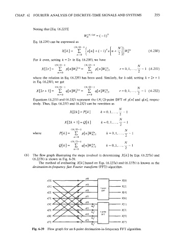
(6) The flow graph illustrating the steps involved in determining X[k] by Eqs. (6.227~) and
(6.2276) is shown in Fig. 6-39.
The method of evaluating X[k] based on Eqs. (6.227~) and (6.2276) is known as the
decimation-in-frequency fast Fourier transform (FFT) algorithm.

Fig. 6-39 Flow graph for an &point decimation-in-frequency FFT algorithm.