Page 369 - Schaum's Outline of Theory and Problems of Signals and Systems

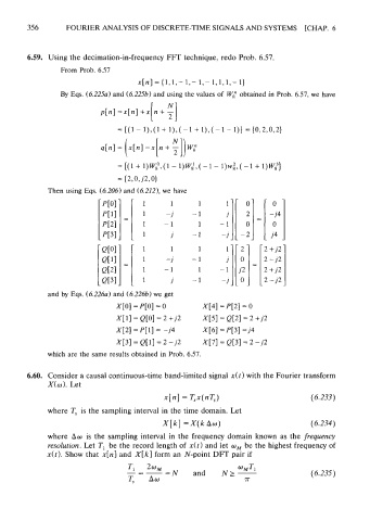
356 FOURIER ANALYSIS OF DISCRETE-TIME SIGNALS AND SYSTEMS [CHAP. 6

6.59. Using the decimation-in-frequency FFT technique, redo Prob. 6.57.
From Prob. 6.57

x[n]=(l,l,-1,-1,-l,l,l,-1)
By Eqs. (6.225a) and (6.225b) and using the values of W," obtained in Prob. 6.57, we have

= (2,0, 12,O)
Then using Eqs. (6.206) and (6.212). we have

and by Eqs. (6.226a) and (6.2266) we get
X[0] = P[0] = 0 X[4] = P[2] =o

X[1] = Q[O] = 2 + j2 X[5] = Q[2] = 2 + j2
X[2] = P[1] = -j4 X[6] = P[3] = j4
X[3] = Q[l] = 2 - j2 X[7] = Q[3] = 2 - j2
which are the same results obtained in Prob. 6.57.

6.60. Consider a causal continuous-time band-limited signal x(t) with the Fourier transform
X(w). Let

where Ts is the sampling interval in the time domain. Let
X[k] = X(k Aw)

where Aw is the sampling interval in the frequency domain known as the frequency
resolution. Let T, be the record length of x(t) and let w, be the highest frequency of
x(t). Show that x[n] and X[k] form an N-point DFT pair if
TI 2% w~T1
-=- =N and N2-
T, Aw T