Page 387 - Schaum's Outline of Theory and Problems of Signals and Systems

374 STATE SPACE ANALYSIS [CHAP. 7

7.6 SOLUTIONS OF STATE EQUATIONS FOR CONTINUOUS-TIME LTI SYSTEMS
A. Laplace Transform Method:

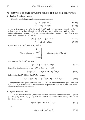
Consider an N-dimensional state space representation

where A, b, c, and d are N x N, N X 1, 1 X N, and 1 X 1 matrices, respectively. In the
following we solve Eqs. (7.46~) and (7.46b) with some initial state q(0) by using the
unilateral Laplace transform. Taking the unilateral Laplace transform of Eqs. (7.46~) and
(7.466) and using Eq. (3.441, we get

Rearranging Eq. (7.47~1, we have

(sI - A)Q(s) = q(0) + bX(s)

Premultiplying both sides of Eq. (7.48) by (sI - A)-' yields
Q(S) = (SI- A)-'~(o) + (SI- A)-'~x(s) (7.49)

Substituting Eq. (7.49) into Eq. (7.47b1, we get

Taking the inverse Laplace transform of Eq. (7.501, we obtain the output y(t). Note that
c(sI - A)-'q(0) corresponds to the zero-input response and that the second term corre-
sponds to the zero-state response.

B. System Function H(s):
As in the discrete-time case, the system function H(s) of a continuous-time LTI system
is defined by H(s) = Y(s)/X(s) with zero initial conditions. Thus, setting q(0) = 0 in
Eq. (7.501, we have

Thus,